Facial Emotion Expressions
In this assignment, we are given a dataset of images containing various facial emotions. There are 7 different categories. Our goal is to classify the test dataset into one of these categories. I used Convolutional neural network (CNN) model to classify the images.
Convolutional neural network (CNN): CNN is an artificial neural network(ANN) which is mostly used in image classification. There are some disadvantages of using ANN for image classification. They are it involves too much computation, treats local pixels same as pixels far apart and sensitive to location of an object in an image. To overcome these problems, we use CNN. CNN uses filters to detect features in images. Filters are rotated throughout the whole image to detect features. After applying the filters over the image, we get feature maps. This whole process is convolution layer. We will use Relu activation function to the obtained feature maps. Relu helps with making model non-linear. Next pooling layer is applied to reduce the size to reduce computations. There could be any number of convolution and pooling layers. After that we will connect these to fully connected dense layer. CNN does not take care of rotation and scale. We have to use data augmentation techniques to generate new rotated, scaled images from existing dataset. As hyperparameters we have to specify how many filters to be used and size of each filter. [1]
Coding part: I used the entire code from Kaggle to read the data, perform transformation, perform augmentation, defining the model and fitting the model.[2]
Code:
from tensorflow.keras.applications import EfficientNetB2
backbone = EfficientNetB2(
input_shape=(96, 96, 3),
include_top=False
)
model = tf.keras.Sequential([
backbone,
tf.keras.layers.Conv2D(128, 3, padding='same', activation='relu'),
tf.keras.layers.GlobalAveragePooling2D(),
tf.keras.layers.Dense(128, activation='relu'),
tf.keras.layers.Dropout(0.3),
tf.keras.layers.Dense(7, activation='softmax')
])
model.compile(
optimizer=tf.keras.optimizers.Adam(learning_rate=0.001, beta_1=0.9, beta_2=0.999, epsilon=1e-07),
loss = 'categorical_crossentropy',
metrics=['accuracy' , tf.keras.metrics.Precision(name='precision'),tf.keras.metrics.Recall(name='recall')]
)
early_stopping=tf.keras.callbacks.EarlyStopping(monitor="accuracy",patience=2,mode="auto")
history = model.fit(
train_dataset,
steps_per_epoch=len(train_labels)//BATCH_SIZE,
epochs=12,
callbacks=[early_stopping],
validation_data=val_dataset,
validation_steps = len(valid_labels)//BATCH_SIZE,
class_weight=class_weight
)
This the model building code. The output is.
Epoch 1/12
450/450 [==============================] - 2457s 5s/step - loss: 2.8624 - accuracy: 0.8298 - precision: 0.8705 - recall: 0.7791 - val_loss: 11.7143 - val_accuracy: 0.1115 - val_precision: 0.1115 - val_recall: 0.1115
Epoch 2/12
450/450 [==============================] - 2598s 6s/step - loss: 1.9127 - accuracy: 0.8024 - precision: 0.8529 - recall: 0.7319 - val_loss: 11.7697 - val_accuracy: 0.1115 - val_precision: 0.1115 - val_recall: 0.1115
Epoch 3/12
450/450 [==============================] - 2494s 6s/step - loss: 1.5994 - accuracy: 0.8158 - precision: 0.8509 - recall: 0.7600 - val_loss: 19.6663 - val_accuracy: 0.1109 - val_precision: 0.1109 - val_recall: 0.1109
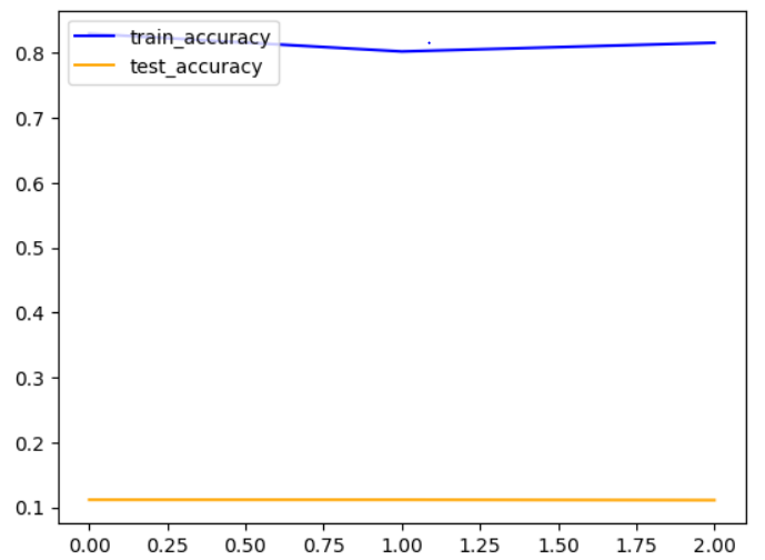
The training accuracy is 0.8158 and testing accuracy is 0.1109. I plotted a graph for this.
Code:
plt.plot(history.history['accuracy'],color='blue',label='train_accuracy')
plt.plot(history.history['val_accuracy'],color='orange',label='test_accuracy')
plt.legend(loc='upper left')
plt.show() [3]
Output:
Now again I performed second training .
Code:
model.layers[0].trainable = False
checkpoint = tf.keras.callbacks.ModelCheckpoint("best_weights.h5",verbose=1,save_best_only=True,save_weights_only = True)
early_stop = tf.keras.callbacks.EarlyStopping(monitor="accuracy",patience=2)
history = model.fit(
train_dataset,
steps_per_epoch=len(train_labels)//BATCH_SIZE,
epochs=8,
callbacks=[checkpoint , early_stop],
validation_data=val_dataset,
validation_steps = len(valid_labels)//BATCH_SIZE,
class_weight=class_weight
)
Output:
Epoch 1/8
450/450 [==============================] - ETA: 0s - loss: 1.4908 - accuracy: 0.8213 - precision: 0.8572 - recall: 0.7565
Epoch 1: val_loss improved from inf to 28.19199, saving model to best_weights.h5
450/450 [==============================] - 2384s 5s/step - loss: 1.4908 - accuracy: 0.8213 - precision: 0.8572 - recall: 0.7565 - val_loss: 28.1920 - val_accuracy: 0.1115 - val_precision: 0.1115 - val_recall: 0.1115
Epoch 2/8
450/450 [==============================] - ETA: 0s - loss: 1.5421 - accuracy: 0.7991 - precision: 0.8530 - recall: 0.7368
Epoch 2: val_loss improved from 28.19199 to 18.80349, saving model to best_weights.h5
450/450 [==============================] - 2400s 5s/step - loss: 1.5421 - accuracy: 0.7991 - precision: 0.8530 - recall: 0.7368 - val_loss: 18.8035 - val_accuracy: 0.1119 - val_precision: 0.1119 - val_recall: 0.1119
Epoch 3/8
450/450 [==============================] - ETA: 0s - loss: 1.4314 - accuracy: 0.7860 - precision: 0.8340 - recall: 0.7267
Epoch 3: val_loss improved from 18.80349 to 13.04038, saving model to best_weights.h5
450/450 [==============================] - 2675s 6s/step - loss: 1.4314 - accuracy: 0.7860 - precision: 0.8340 - recall: 0.7267 - val_loss: 13.0404 - val_accuracy: 0.1112 - val_precision: 0.1112 - val_recall: 0.1112
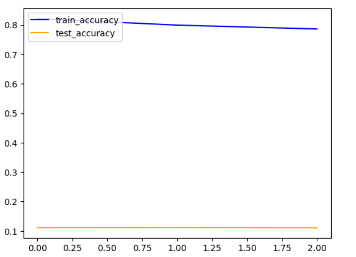
The training accuracy is 0.7860 and testing accuracy is 0.1112. I plotted a graph for this.
Code:
plt.plot(history.history['accuracy'],color='blue',label='train_accuracy')
plt.plot(history.history['val_accuracy'],color='orange',label='test_accuracy')
plt.legend(loc='upper left')
plt.show()
Output:
Now I changed the parameter values. I increased filters to 256, changed kernel size to (4,4). I used max pooling and increased dense layers to 256. Now the new model is
Code:
from tensorflow.keras import models,layers
cnn=models.Sequential([
layers.Conv2D(filters=256,kernel_size=(4,4),activation='relu',input_shape=(96,96,3)),
layers.MaxPooling2D((3,3)),
layers.Conv2D(filters=256,kernel_size=(4,4),activation='relu',input_shape=(96,96,3)),
layers.MaxPooling2D((3,3)),
layers.Flatten(),
layers.Dense(256,activation='relu'),
layers.Dense(7,activation='relu')
])
early_stopping=tf.keras.callbacks.EarlyStopping(monitor="accuracy",patience=2,mode="auto")
cnn.compile(
optimizer='adam',
loss = 'categorical_crossentropy',
metrics=['accuracy' , tf.keras.metrics.Precision(name='precision'),tf.keras.metrics.Recall(name='recall')]
)
history1 = cnn.fit(
train_dataset,
steps_per_epoch=len(train_labels)//BATCH_SIZE,
epochs=12,
callbacks=[early_stopping],
validation_data=val_dataset,
validation_steps = len(valid_labels)//BATCH_SIZE,
class_weight=class_weight
)
Output:
Epoch 1/12
450/450 [==============================] - 3057s 7s/step - loss: nan - accuracy: 0.1342 - precision: 0.0000e+00 - recall: 0.0000e+00 - val_loss: nan - val_accuracy: 0.1364 - val_precision: 0.0000e+00 - val_recall: 0.0000e+00
Epoch 2/12
450/450 [==============================] - 3066s 7s/step - loss: nan - accuracy: 0.1389 - precision: 0.0000e+00 - recall: 0.0000e+00 - val_loss: nan - val_accuracy: 0.1364 - val_precision: 0.0000e+00 - val_recall: 0.0000e+00
Epoch 3/12
450/450 [==============================] - 3093s 7s/step - loss: nan - accuracy: 0.1389 - precision: 0.0000e+00 - recall: 0.0000e+00 - val_loss: nan - val_accuracy: 0.1364 - val_precision: 0.0000e+00 - val_recall: 0.0000e+00
Epoch 4/12
450/450 [==============================] - 3362s 7s/step - loss: nan - accuracy: 0.1389 - precision: 0.0000e+00 - recall: 0.0000e+00 - val_loss: nan - val_accuracy: 0.1364 - val_precision: 0.0000e+00 - val_recall: 0.0000e+00
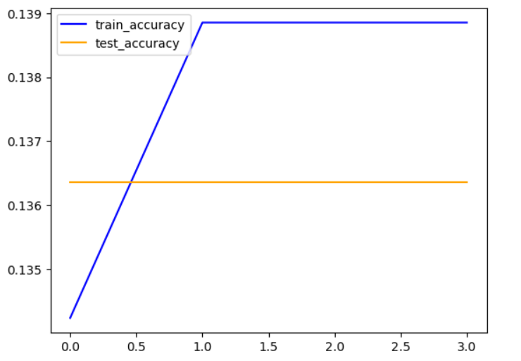
The training accuracy is 0.1389 and testing accuracy is 0.1364. I plotted a graph for this.
Code:
plt.plot(history1.history['accuracy'],color='blue',label='train_accuracy')
plt.plot(history1.history['val_accuracy'],color='orange',label='test_accuracy')
plt.legend(loc='upper left')
plt.show()
Output:
Now again I performed second training .
Code:
cnn.layers[0].trainable = False
checkpoint = tf.keras.callbacks.ModelCheckpoint("best_weights.h5",verbose=1,save_best_only=True,save_weights_only = True)
early_stop = tf.keras.callbacks.EarlyStopping(monitor="accuracy",patience=2)
history1 = cnn.fit(
train_dataset,
steps_per_epoch=len(train_labels)//BATCH_SIZE,
epochs=8,
callbacks=[checkpoint , early_stop],
validation_data=val_dataset,
validation_steps = len(valid_labels)//BATCH_SIZE,
class_weight=class_weight
)
Output:
Epoch 1/8
450/450 [==============================] - ETA: 0s - loss: nan - accuracy: 0.1386 - precision: 0.0000e+00 - recall: 0.0000e+00
Epoch 1: val_loss did not improve from inf
450/450 [==============================] - 3567s 8s/step - loss: nan - accuracy: 0.1386 - precision: 0.0000e+00 - recall: 0.0000e+00 - val_loss: nan - val_accuracy: 0.1364 - val_precision: 0.0000e+00 - val_recall: 0.0000e+00
Epoch 2/8
450/450 [==============================] - ETA: 0s - loss: nan - accuracy: 0.1389 - precision: 0.0000e+00 - recall: 0.0000e+00
Epoch 2: val_loss did not improve from inf
450/450 [==============================] - 2849s 6s/step - loss: nan - accuracy: 0.1389 - precision: 0.0000e+00 - recall: 0.0000e+00 - val_loss: nan - val_accuracy: 0.1364 - val_precision: 0.0000e+00 - val_recall: 0.0000e+00
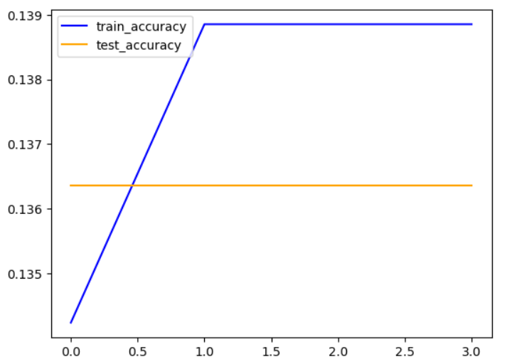
The training accuracy is 0.1389 and testing accuracy is 0.1364. I plotted a graph for this.
Code:
plt.plot(history1.history['accuracy'],color='blue',label='train_accuracy')
plt.plot(history1.history['val_accuracy'],color='orange',label='test_accuracy')
plt.legend(loc='upper left')
plt.show()
Output:
Contribution:
I changed the number of filters, increased kernel size , used max pooling, increased dense layers and also plotted graphs.
References:
1] I watched explanation of CNN video in you tube. The link to the video is (7) Simple explanation of convolutional neural network | Deep Learning Tutorial 23 (Tensorflow & Python) - YouTube
3] I referred you tube video to plot graphs. The link is (7) Build a Deep CNN Image Classifier with ANY Images - YouTube